Time-Series Forecasting using ARIMA model

Introduction

A time-series is a series of data points measured at consistent time intervals. This time interval may be hourly, daily, weekly, monthly, quarterly, yearly and so on. In a time series, each data point is dependent on the previous data points. Time-series patterns may be classified as:

• Trend – Exists when there is a long-term increase or decrease in the data
• Seasonal – Occurs when time series is of a fixed and known frequency
• Cyclic – Occurs when the time series is not of a fixed frequency

Forecasting is defined as the process of making predictions of the future based on the past and present data and by analysis of trends. Time-series forecasting is the process of using a model to predict future values based on previously-observed values. ARIMA is a very popular technique for time-series modelling.

ARIMA (Auto Regressive Integrated Moving Average) is like a linear regression equation where the predictors depend on the following parameters:

• p (lag order) – number of lag observations included in the model
• d (degree of differencing) – number of times the raw observations are differenced
• q (order of moving average) – size of the moving average window

ARIMA can be used in cases where the data is stationary, does not contain any anomaly and is uni-variate. Cases of non-stationarity can be eliminated by applying differencing once or twice.

Model Implementation

• Plot, examine and prepare the time-series for modelling.
• Extract the seasonality component from the time-series.
• Test for stationarity and apply appropriate transformations.
• Choose the best fit for the ARIMA model.
• Forecast the time-series.

The process of extracting trend, seasonality and cycle from a time-series is referred to as decomposition. Deconstruction of the data helps to understand its behaviour and prepare a foundation for building the forecast model. Decomposition is done in Python using seasonal_decompose().

ACF (Auto-correlation) plots help in determining the lag order (q) of the model.

PACF (Partial Auto-correlation) plots help in determining the order of moving average (p) of the model.

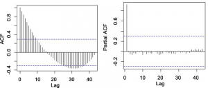
Sample ACF & PACF plots

Auto arima function helps to identify the optimised fit ARIMA model. The .fit() command is used to fit the model without having to select p, d & q values. ARIMA takes into account the AIC and BIC values generated to determine the best combination of parameters.

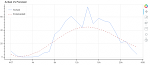
Graphical representation of the ARIMA model

Conclusion

ARIMA is the simplest technique for performing time-series forecasting. ARIMA models are more flexible than other statistical models such as exponential smoothing or linear regression and do not over-fit.